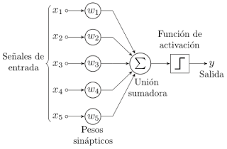
The article (introduction to the perceptron) shows the perceptron with the activation function, which in the figure is a square wave, but it can also be another type of function.
The article (building a neural network in a few minutes) shows the activation function called sigmoid.

And the article (A Neural Network for supervised learning using Scikit-learn) uses the tanh function.
Scikit-learn's multi-layer perceptron supports several types of activation functions (documentation), such as:
- identity: The activation function is
f(x)=x. - logistic: The activation function is the sigmoid function
f(x)=1/(1+exp(-x)). - tanh: The activation function is the hyperbolic tangent function
f(x)=tanh(x). - relu: The activation function is the rectified linear unit function
f(x)=max(0,x).
The code will show the different functions and their plots; then the neural network from the article A Neural Network for supervised learning using Scikit-learn is taken, using different activation functions: the neuron is trained with each activation function and we try to predict the result.
Here is the code:
In [1]:
#Se importa numpy y matplotlib
import matplotlib.pyplot as plt
import numpy as np
%matplotlib inline
In [2]:
#Se define el rango de valores
z = np.linspace(-10,10,100)
In [3]:
#Onda cuadrada
def cuadrada(z):
    return 1*(z>0)
In [4]:
#Se calcula la onda cuadrada a partir del rango de valores
a = cuadrada(z)
In [5]:
#Se gráfica la onda cuadrada
plt.plot(z,a)
Out[5]:
[<matplotlib.lines.Line2D at 0x7f90ba52c278>]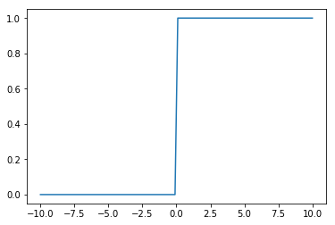
In [6]:
#Se define la función Identidad
def identidad(z):
    return z
In [7]:
#Se calcula la función identidad a partir del rango de valores
b = identidad(z)
In [8]:
#Se gráfica.
plt.plot(z,b)
Out[8]:
[<matplotlib.lines.Line2D at 0x7f90ba49e7f0>]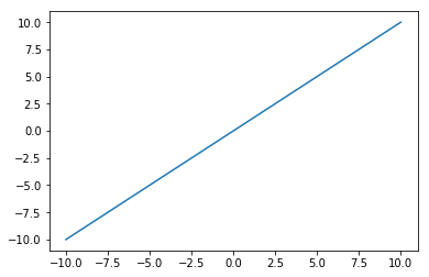
In [9]:
#Función ReLU
def ReLU(z):
    return z * (z > 0)
In [10]:
#Se calcula la función ReLU a partir del rango de valores
c = ReLU(z)
In [11]:
#Se gráfica la función
plt.plot(z,c)
Out[11]:
[<matplotlib.lines.Line2D at 0x7f90ba46c6d8>]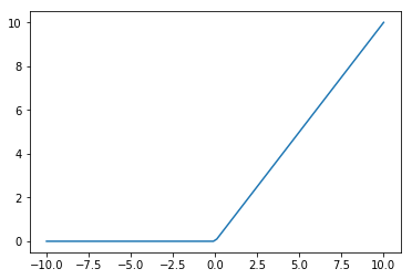
In [12]:
#Función tangente hiperbolico
def tanh(z):
    return(np.exp(z)-np.exp(-z))/(np.exp(z)+np.exp(-z))
In [13]:
#Se calcula la tangente hiperbolica a partir del rango de valores
d = tanh(z)
In [14]:
#Se gráfica
plt.plot(z,d)
Out[14]:
[<matplotlib.lines.Line2D at 0x7f90ba42e550>]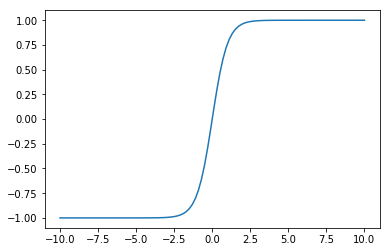
In [15]:
#Función sigmoide
def sigmoide(z):
    return 1/(1+np.exp(-z))
In [16]:
#Se calcula la sigmoide a partir del rango de valores
e = sigmoide(z)
In [17]:
#Se gráfica la función
plt.plot(z,e)
Out[17]:
[<matplotlib.lines.Line2D at 0x7f90ba3f0be0>]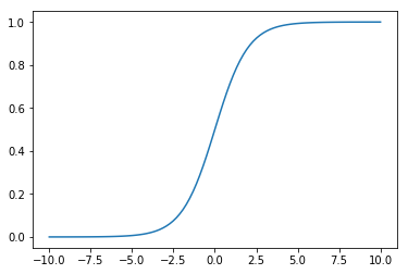
The difference between the activation functions is how smooth or not each curve is. That is, how abrupt its slope is, or the derivative of the function.
Next, a neural network is created using scikit-learn
In [18]:
#Se importa de la red neuronal MLPClassifier
from sklearn.neural_network import MLPClassifier
In [19]:
#Se definen los datos de entrada
datos_entrada = np.array([
    0, 0,
    0, 1,
    1, 0,
    1, 1
]).reshape(4, 2)
In [20]:
#Se definen los datos de salida
datos_salida = np.array([0, 1, 1, 0]).reshape(4,)
In [21]:
#Se crea la red neuronal con función de activación relu y 100 mil iteraciones
model = MLPClassifier(activation='relu', max_iter=100000, hidden_layer_sizes=(4,2))
In [22]:
#Se entrena a la red neuronal
model.fit(datos_entrada,datos_salida)
Out[22]:
MLPClassifier(activation='relu', alpha=0.0001, batch_size='auto', beta_1=0.9,
       beta_2=0.999, early_stopping=False, epsilon=1e-08,
       hidden_layer_sizes=(4, 2), learning_rate='constant',
       learning_rate_init=0.001, max_iter=100000, momentum=0.9,
       nesterovs_momentum=True, power_t=0.5, random_state=None,
       shuffle=True, solver='adam', tol=0.0001, validation_fraction=0.1,
       verbose=False, warm_start=False)
In [23]:
#Se hace la predicción
print('prediccion:', model.predict(datos_entrada))

prediccion: [0 1 0 1]
The result returned by the neural network should be [0,1,1,0] and it returns [0,1,0,1], which is wrong. The neural network is built again, but now using the identity activation function.
In [24]:
model = MLPClassifier(activation='identity', max_iter=100000, hidden_layer_sizes=(4,2))In [25]:
#Se entrena a la red neuronal
model.fit(datos_entrada,datos_salida)
Out[25]:
MLPClassifier(activation='identity', alpha=0.0001, batch_size='auto',
       beta_1=0.9, beta_2=0.999, early_stopping=False, epsilon=1e-08,
       hidden_layer_sizes=(4, 2), learning_rate='constant',
       learning_rate_init=0.001, max_iter=100000, momentum=0.9,
       nesterovs_momentum=True, power_t=0.5, random_state=None,
       shuffle=True, solver='adam', tol=0.0001, validation_fraction=0.1,
       verbose=False, warm_start=False)
In [26]:
#Se hace la predicción
print('prediccion:', model.predict(datos_entrada))

prediccion: [0 0 0 0]
The result returned by the neural network should be [0,1,1,0] and it returns [0,0,0,0], which is wrong. The neural network is built again, but now using the sigmoid activation function (logistic).
In [27]:
model = MLPClassifier(activation='logistic', max_iter=100000, hidden_layer_sizes=(4,2))In [28]:
#Se entrena a la red neuronal
model.fit(datos_entrada,datos_salida)
Out[28]:
MLPClassifier(activation='logistic', alpha=0.0001, batch_size='auto',
       beta_1=0.9, beta_2=0.999, early_stopping=False, epsilon=1e-08,
       hidden_layer_sizes=(4, 2), learning_rate='constant',
       learning_rate_init=0.001, max_iter=100000, momentum=0.9,
       nesterovs_momentum=True, power_t=0.5, random_state=None,
       shuffle=True, solver='adam', tol=0.0001, validation_fraction=0.1,
       verbose=False, warm_start=False)
In [29]:
#Se hace la predicción
print('prediccion:', model.predict(datos_entrada))

prediccion: [1 1 1 1]
The result returned by the neural network should be [0,1,1,0] and it returns [1,1,1,1], which is wrong. The neural network is built again, but now using the tanh activation function.
In [33]:
model = MLPClassifier(activation='tanh', max_iter=100000, hidden_layer_sizes=(4,2))In [34]:
#Se entrena a la red neuronal
model.fit(datos_entrada,datos_salida)
Out[34]:
MLPClassifier(activation='tanh', alpha=0.0001, batch_size='auto', beta_1=0.9,
       beta_2=0.999, early_stopping=False, epsilon=1e-08,
       hidden_layer_sizes=(4, 2), learning_rate='constant',
       learning_rate_init=0.001, max_iter=100000, momentum=0.9,
       nesterovs_momentum=True, power_t=0.5, random_state=None,
       shuffle=True, solver='adam', tol=0.0001, validation_fraction=0.1,
       verbose=False, warm_start=False)
In [35]:
#Se hace la predicción
print('prediccion:', model.predict(datos_entrada))

prediccion: [0 1 1 0]
The result returned by the neural network should be [0,1,1,0] and it returns [0,1,1,0], which is the expected result. This shows that it is very important to select the right activation function when defining a neural network and training it.
Make a donation! If you liked the article you can make a donation with Bitcoin (BTC) using the digital wallet of your choice to the following address: 17MtNybhdkA9GV3UNS6BTwPcuhjXoPrSzV
Or by scanning the QR code from the wallet: