A mean response time of 393 milliseconds does not say whether every request takes that long or whether most take 300 and a few go past a second. To see it you have to draw the distribution, not the mean.
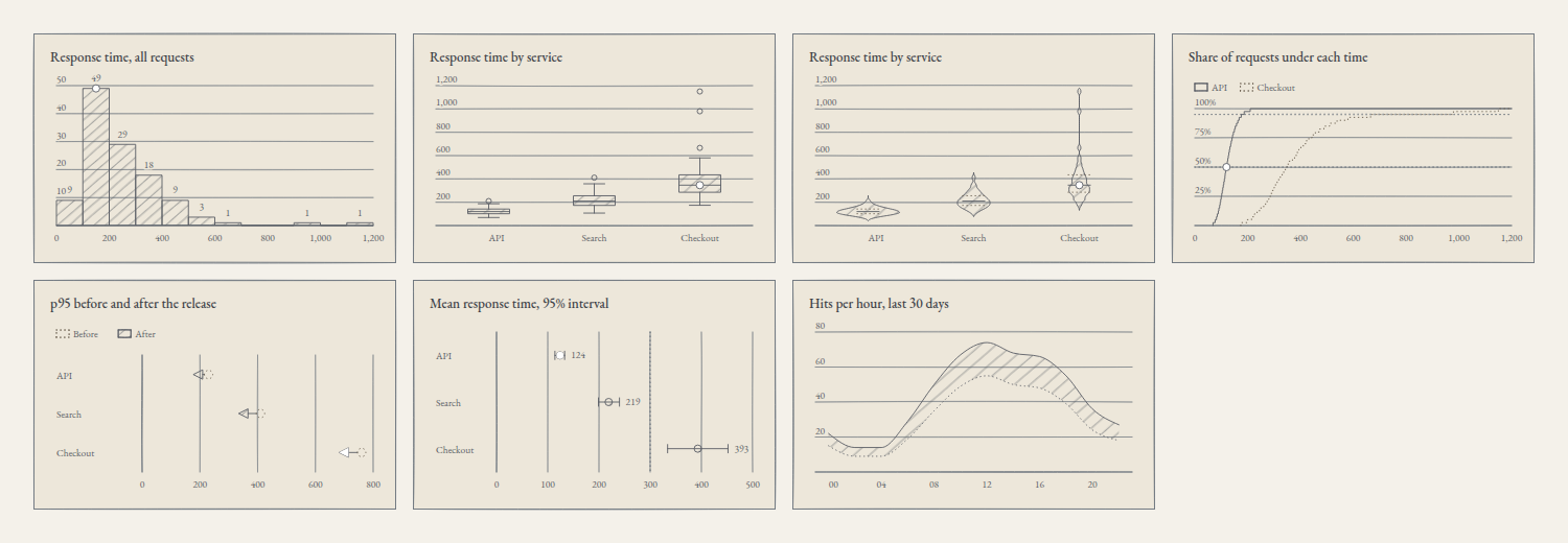
This level 2 article of the series on silverpoint adds the response times of three services to the operations panel. It draws them with the distribution charts, compares a before and an after, and shows the uncertainty of an estimate. They are charts of the distributions-comparisons family and of the areas family, the ones from article 08.
The data
Forty response times in milliseconds per service: API, Search and Checkout. Distribution charts take one row per observation, so the times are written per service and flattened. In src/latency.ts:
export type Timing = { service: string; ms: number };

const samples: Record<string, number[]> = {
  API: [69, 115, 158, 104, 138, 91, 125, 210, 114, 153, 102, 136, 89, 123, 187, 112, 150, 100, 133, 85,
    121, 176, 110, 146, 98, 131, 82, 119, 168, 108, 143, 96, 129, 77, 117, 163, 106, 141, 94, 127],
  Search: [107, 200, 291, 177, 248, 151, 220, 411, 197, 282, 174, 243, 146, 216, 358, 193, 274, 169, 238, 140,
    212, 333, 189, 267, 165, 233, 133, 208, 315, 185, 260, 161, 229, 123, 204, 302, 181, 254, 156, 224],
  Checkout: [174, 324, 472, 287, 402, 245, 356, 666, 318, 457, 281, 394, 236, 350, 580, 312, 444, 274, 386, 226,
    343, 539, 306, 432, 268, 378, 215, 337, 511, 300, 421, 261, 370, 199, 331, 489, 294, 411, 980, 1150],
};

export const timings: Timing[] = Object.entries(samples).flatMap(([service, values]) =>
  values.map((ms) => ({ service, ms })),
);
The result is 120 rows such as { service: 'Checkout', ms: 980 }. The last two of Checkout are requests that went past a second.
Four ways to see a distribution
In src/Distributions.tsx:
import { BoxPlotChart } from '@silverpoint/react/box-plot-chart';
import { EcdfChart } from '@silverpoint/react/ecdf-chart';
import { HistogramChart } from '@silverpoint/react/histogram-chart';
import { ViolinChart } from '@silverpoint/react/violin-chart';
import { timings } from './latency';

const twoServices = timings.filter((row) => row.service !== 'Search');

export function Distributions() {
  return (
    <>
      <HistogramChart data={timings} valueKey="ms" bins={12} title="Response time, all requests" />
      <BoxPlotChart data={timings} valueKey="ms" groupKey="service" title="Response time by service" />
      <ViolinChart data={timings} valueKey="ms" groupKey="service" title="Response time by service" />
      <EcdfChart
        data={twoServices}
        valueKey="ms"
        groupKey="service"
        markers={[0.5, 0.95]}
        title="Share of requests under each time"
      />
    </>
  );
}
The histogram counts how many observations fall into each interval. bins accepts a number of equal intervals or a list of increasing thresholds. Without bins, the number comes from the Freedman–Diaconis rule, or from Sturges' rule when the interquartile range is 0; with this data that would be 22 intervals of 50 ms. With bins={12} there are twelve of 100 ms, from 0 to 1200. cumulative turns the counts into a running total.
The box plot sums up each group in five numbers: the box runs from the first to the third quartile, the line inside is the median and the whiskers reach the last observation within 1.5 interquartile ranges of the box. Whatever lies beyond is drawn as loose points. In Checkout there are three: 666, 980 and 1150. whisker changes the 1.5 and outliers={false} hides the points.
The violin draws each group's density, mirrored, with the quartiles marked inside. It shows what the box hides: if a group has two modes, the box does not say so and the violin does. bandwidth sets the kernel's width; by default it is the mean of the groups' Silverman rules.
The cumulative distribution (ECDF) draws, for each time, the share of requests that take that long or less. markers draws rules at the quantiles you ask for: here, the median and the 95th percentile. It draws two groups at most, which is why the example filters out Search.
The chart draws derived values
These four charts do not draw your rows, but what they compute from them: intervals and counts, quartiles, densities. silverpoint applies that same rule to everything else:
- The data table shows the derived values. The box plot's has the columns
n,min,q1,median,q3,maxandoutliers, one row per service.minandmaxare the ends of the whiskers: inAPI,maxis 187 and 210 appears inoutliers. - The description names the method and its parameters. The histogram's says "Histogram of 120 ms observations in 12 bins as 12 equal bins, from 0 to 1,200; the fullest bin, 100–200, holds 49".
- Keyboard navigation walks the intervals, or the groups and their outliers, and announces their derived values, not the observations.
- The events hand over a summary. In the box plot, the active item's
datumis{ group, min, q1, median, q3, max, outliers }and itsvalueis the median; in the histogram, thedatumis{ x0, x1, count }.
Two diagnostics belong to these charts, and like every SP0xx, they only appear in development:
SP021: a statistic parameter is not valid and the default is used. Withbins={0}, the histogram falls back to Freedman–Diaconis.SP022: a group has too few observations for its statistic, and they are drawn as points. The box plot needs five per group; the violin, two.
Comparing a before and an after
The service shipped a release, and the question is how much each service's 95th percentile dropped. They are categories with two values, the categories shape with the change intent, and the first in article 08's table is the dumbbell chart.
The uncertainty of an estimate
Each service's mean is an estimate, and it has a margin. The error bar chart draws each estimate with its 95% interval. The dotted line of reference is the latency budget, 300 ms: the mean of Checkout is above it, and its interval does not reach across it.
The band draws uncertainty along an axis: the lowest and highest hits of each two-hour block over the last 30 days.
The three charts take values already computed. In src/summaries.ts:
export type P95Change = { service: string; before: number; after: number };
export type MeanLatency = { service: string; mean: number; low: number; high: number };
export type HitRange = { hour: string; low: number; high: number };

export const p95: P95Change[] = [
  { service: 'API', before: 230, after: 177 },
  { service: 'Search', before: 410, after: 334 },
  { service: 'Checkout', before: 760, after: 682 },
];

export const means: MeanLatency[] = [
  { service: 'API', mean: 124, low: 114, high: 133 },
  { service: 'Search', mean: 219, low: 199, high: 240 },
  { service: 'Checkout', mean: 393, low: 334, high: 452 },
];

export const hitRange: HitRange[] = [
  { hour: '00', low: 15, high: 22 }, { hour: '02', low: 9, high: 14 },
  { hour: '04', low: 9, high: 14 }, { hour: '06', low: 19, high: 29 },
  { hour: '08', low: 35, high: 50 }, { hour: '10', low: 49, high: 67 },
  { hour: '12', low: 55, high: 74 }, { hour: '14', low: 50, high: 68 },
  { hour: '16', low: 48, high: 66 }, { hour: '18', low: 39, high: 55 },
  { hour: '20', low: 24, high: 36 }, { hour: '22', low: 18, high: 27 },
];
The 95th percentiles after the release and the means with their interval come from the times in src/latency.ts. The interval is the mean plus and minus 1.96 standard errors.
In src/Comparisons.tsx:
import { DumbbellChart } from '@silverpoint/react/dumbbell-chart';
import { ErrorBarChart } from '@silverpoint/react/error-bar-chart';
import { RangeBandChart } from '@silverpoint/react/range-band-chart';
import { hitRange, means, p95 } from './summaries';

export function Comparisons() {
  return (
    <>
      <DumbbellChart
        data={p95}
        labelKey="service"
        startKey="before"
        endKey="after"
        names={['Before', 'After']}
        endMarker="arrow"
        title="p95 before and after the release"
      />
      <ErrorBarChart
        data={means}
        labelKey="service"
        estimateKey="mean"
        lowKey="low"
        highKey="high"
        reference={300}
        title="Mean response time, 95% interval"
      />
      <RangeBandChart
        data={hitRange}
        xKey="hour"
        lowKey="low"
        highKey="high"
        title="Hits per hour, last 30 days"
      />
    </>
  );
}| Chart | Accessors | Other props |
|---|---|---|
DumbbellChart | labelKey, startKey, endKey | names, the titles of the two values; endMarker="arrow", an arrow that shows the direction of the change |
ErrorBarChart | labelKey, estimateKey, lowKey, highKey | reference, a dotted rule |
RangeBandChart | xKey, lowKey, highKey | — |
The dumbbell chart and the error bar chart are laid out in rows by default, the way a before and after or a forest plot reads. The descriptions sum up the comparison: the dumbbell chart's says "0 rise, 3 fall; the largest change is Checkout, −78", and the error bars', "read against 300; 0 of them include it".
The two components go together in src/App.tsx:
import { Comparisons } from './Comparisons';
import { Distributions } from './Distributions';

export default function App() {
  return (
    <main className="panel">
      <Distributions />
      <Comparisons />
    </main>
  );
}
The panel class is the grid from article 08.
The code in Reflex
The data, in ops_panel/latency.py:
SAMPLES = {
    "API": [69, 115, 158, 104, 138, 91, 125, 210, 114, 153, 102, 136, 89, 123, 187, 112, 150, 100, 133, 85,
            121, 176, 110, 146, 98, 131, 82, 119, 168, 108, 143, 96, 129, 77, 117, 163, 106, 141, 94, 127],
    "Search": [107, 200, 291, 177, 248, 151, 220, 411, 197, 282, 174, 243, 146, 216, 358, 193, 274, 169, 238, 140,
               212, 333, 189, 267, 165, 233, 133, 208, 315, 185, 260, 161, 229, 123, 204, 302, 181, 254, 156, 224],
    "Checkout": [174, 324, 472, 287, 402, 245, 356, 666, 318, 457, 281, 394, 236, 350, 580, 312, 444, 274, 386, 226,
                 343, 539, 306, 432, 268, 378, 215, 337, 511, 300, 421, 261, 370, 199, 331, 489, 294, 411, 980, 1150],
}

TIMINGS = [{"service": service, "ms": ms} for service, values in SAMPLES.items() for ms in values]

P95 = [
    {"service": "API", "before": 230, "after": 177},
    {"service": "Search", "before": 410, "after": 334},
    {"service": "Checkout", "before": 760, "after": 682},
]

MEANS = [
    {"service": "API", "mean": 124, "low": 114, "high": 133},
    {"service": "Search", "mean": 219, "low": 199, "high": 240},
    {"service": "Checkout", "mean": 393, "low": 334, "high": 452},
]

HIT_RANGE = [
    {"hour": "00", "low": 15, "high": 22}, {"hour": "02", "low": 9, "high": 14},
    {"hour": "04", "low": 9, "high": 14}, {"hour": "06", "low": 19, "high": 29},
    {"hour": "08", "low": 35, "high": 50}, {"hour": "10", "low": 49, "high": 67},
    {"hour": "12", "low": 55, "high": 74}, {"hour": "14", "low": 50, "high": 68},
    {"hour": "16", "low": 48, "high": 66}, {"hour": "18", "low": 39, "high": 55},
    {"hour": "20", "low": 24, "high": 36}, {"hour": "22", "low": 18, "high": 27},
]
The page, in ops_panel/ops_panel.py:
import reflex as rx
from reflex_silverpoint_react import (
    box_plot_chart,
    dumbbell_chart,
    ecdf_chart,
    error_bar_chart,
    histogram_chart,
    range_band_chart,
    violin_chart,
)

from .latency import HIT_RANGE, MEANS, P95, TIMINGS

TWO_SERVICES = [row for row in TIMINGS if row["service"] != "Search"]


def index() -> rx.Component:
    return rx.grid(
        histogram_chart(data=TIMINGS, value_key="ms", bins=12, title="Response time, all requests"),
        box_plot_chart(data=TIMINGS, value_key="ms", group_key="service", title="Response time by service"),
        violin_chart(data=TIMINGS, value_key="ms", group_key="service", title="Response time by service"),
        ecdf_chart(
            data=TWO_SERVICES,
            value_key="ms",
            group_key="service",
            markers=[0.5, 0.95],
            title="Share of requests under each time",
        ),
        dumbbell_chart(
            data=P95,
            label_key="service",
            start_key="before",
            end_key="after",
            names=["Before", "After"],
            end_marker="arrow",
            title="p95 before and after the release",
        ),
        error_bar_chart(
            data=MEANS,
            label_key="service",
            estimate_key="mean",
            low_key="low",
            high_key="high",
            reference=300,
            title="Mean response time, 95% interval",
        ),
        range_band_chart(
            data=HIT_RANGE,
            x_key="hour",
            low_key="low",
            high_key="high",
            title="Hits per hour, last 30 days",
        ),
        columns="4",
        gap="16px",
        padding="32px",
    )


app = rx.App()
app.add_page(index)
The descriptions and the data tables are the same as in React: the engine does the computing, not the adapter.
In Vue and in Angular
| Chart | Vue | Angular |
|---|---|---|
| Histogram | SpHistogramChart | <sp-histogram-chart> |
| Box plot | SpBoxPlotChart | <sp-box-plot-chart> |
| Violin | SpViolinChart | <sp-violin-chart> |
| Cumulative distribution | SpEcdfChart | <sp-ecdf-chart> |
| Dumbbell | SpDumbbellChart | <sp-dumbbell-chart> |
| Error bars | SpErrorBarChart | <sp-error-bar-chart> |
| Band | SpRangeBandChart | <sp-range-band-chart> |
Each one is imported from its own path, such as @silverpoint/vue/box-plot-chart or @silverpoint/angular/box-plot-chart, and the props are the same with each framework's syntax.
What comes next
The panel now shows the shape of the response times, not just their mean. Article 15 closes level 2 with the data that does not fit a flat table: hierarchies, flows and networks, and the level navigation of the hierarchical charts.
The gallery shows the 14 charts of the distributions and comparisons family.