This article shows an introduction to the Streamlit framework using an old post, Plotting electric field lines with matplotlib and Python.

Streamlit

Streamlit is a framework that aims to be the fastest way to create and share data apps.

You can find its documentation at the following link.

Installation

To install streamlit, use pip and run a base example:

pip install streamlit
streamlit hello

When streamlit is run, a web server is started on port 8501, as shown below:

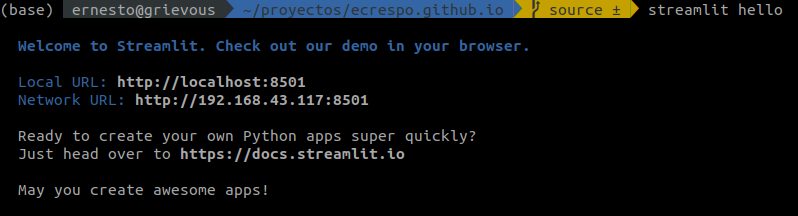
When you open the link you get an initial page like the one shown below:

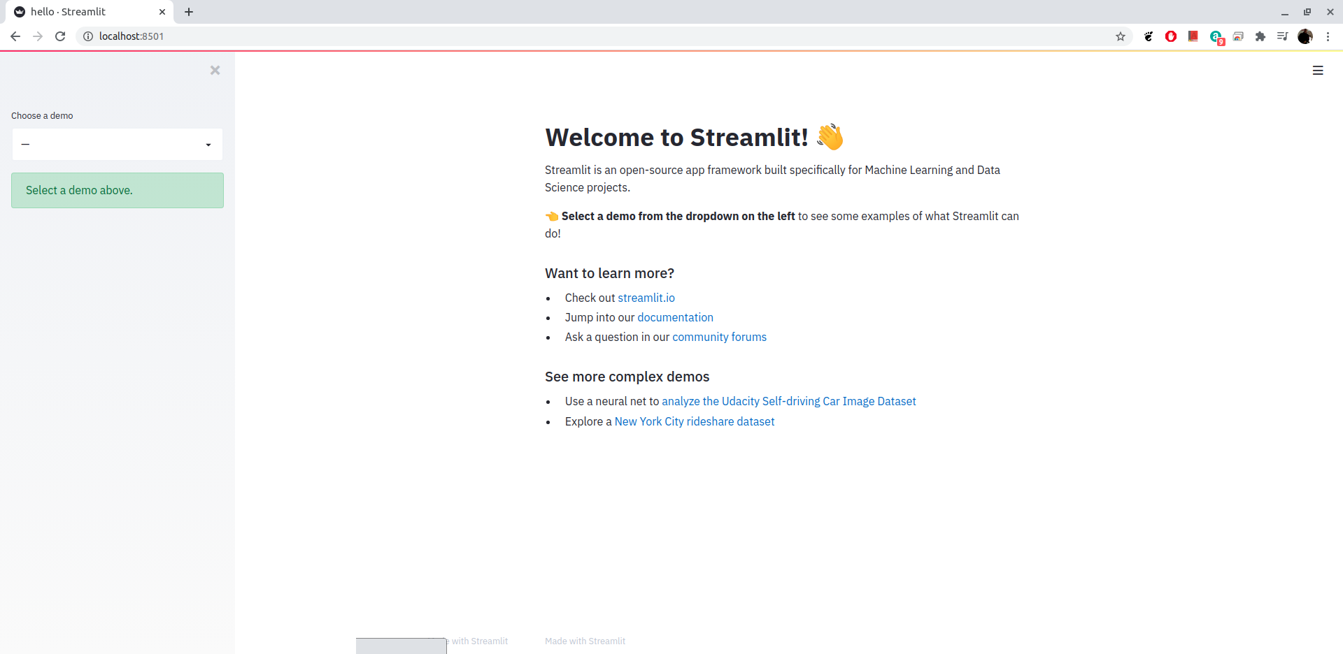
And it has several demos like the following:

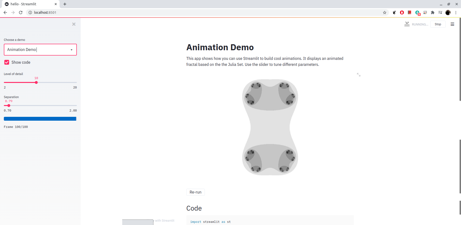
Magnetic Field Visualization with Python and Streamlit

As mentioned before, this post is based on a previous article about magnetic field visualization with Python and matplotlib. You can see the source code on github or the notebook.

A future article will give an introduction to the different components of Streamlit; for now, the magnetic field visualization code will be shown as a webapp in the simplest way possible.

The file structure of the repository is the following:

.
├── app.py
├── LICENSE
├── README.md
└── requirements.txt

The code of app.py is shown below:

import matplotlib.pyplot as plt
import numpy as np
import streamlit as st
from matplotlib.patches import Circle

# https://github.com/ecrespo/codigo_blog/blob/master/graficacion/campoelectric/graficar%2Bcampo%2Belectrico.ipynb
# https://github.com/ecrespo/codigo_blog/blob/master/graficacion/campoelectric/graficar%2Bcampo%2Belectrico.py
# https://www.seraph.to/blog/graficarlineasdecampoelectricoconmatplotlibypython


@st.cache(allow_output_mutation=True)
def magnetic_field_e(q, r0, x, y) -> tuple:
    """Retorna el vector de campo eléctrico E=(Ex,Ey) de una carga q en r0"""
    den = np.hypot(x - r0[0], y - r0[1]) ** 3
    return q * (x - r0[0]) / den, q * (y - r0[1]) / den


@st.cache(allow_output_mutation=True)
def magnetic_field_vector(n: int, axis_x: int, axis_y: int) -> dict:
    """Cálculo del campo electromagnetico según la cantidad de dipolos.

    Args:
        n (int): Número de cargas para definir el dipolo

    Returns:
        dict: x,y,charges,Ex,Ey
    """
    # # puntos de los ejes x e y.
    nx, ny = 128, 128
    x = np.linspace(-axis_x, axis_x, nx)
    y = np.linspace(-axis_y, axis_y, ny)
    X, Y = np.meshgrid(x, y)
    # # Crear un multipolo con nq cargas
    # count = número de q. En ese caso es 1 dipolo
    count = n
    nq = 2 ** int(count)
    charges = [
        (i % 2 * 2 - 1, (np.cos(2 * np.pi * i / nq), np.sin(2 * np.pi * i / nq)))
        for i in range(nq)
    ]

    # # Vector de campo eléctrico como componentes separados (Ex,Ey)
    Ex, Ey = np.zeros((ny, nx)), np.zeros((ny, nx))
    for charge in charges:
        ex, ey = magnetic_field_e(*charge, x=X, y=Y)
        Ex += ex
        Ey += ey

    return {"x": x, "y": y, "charges": charges, "Ex": Ex, "Ey": Ey}


def main():
    """Generación de la webapp con streamlit"""
    # Definir título
    st.title("Magnetic fields")
    # Entrada de datos en el sidebar.
    st.sidebar.header("Inputs:")
    # min: 1, max: 5, default: 1
    n = int(st.sidebar.slider("Charges", 1, 10, 1))
    # SelectBox en sidebar
    min_max_scale = int(
        st.sidebar.selectbox("min,max value in graph", list(range(11, 21)))
    )
    # Graficar usando matplotlib
    fig = plt.figure()
    ax = fig.add_subplot(111)
    # Se realiza el cálculod el vector de campo magnético.
    res = magnetic_field_vector(n, min_max_scale, min_max_scale)
    # Muestra la cantidad de polos que se definen en la entrada de datos.
    st.header(f"{2*n} Polos")
    # Dibujar las líneas de flujo con mapa de colores y estilos apropiados.
    color = 2 * np.log(np.hypot(res["Ex"], res["Ey"]))
    ax.streamplot(
        res["x"],
        res["y"],
        res["Ex"],
        res["Ey"],
        color=color,
        linewidth=1,
        cmap=plt.cm.inferno,
        density=2,
        arrowstyle="->",
        arrowsize=1.5,
    )
    # Agregar circulos para las cargas.
    charge_colors = {True: "#aa0000", False: "#0000aa"}

    for q, pos in res["charges"]:
        ax.add_artist(Circle(pos, 0.05, color=charge_colors[q > 0]))

    # Graficar
    ax.set_xlabel("$x$")
    ax.set_ylabel("$y$")
    ax.set_xlim(-min_max_scale, min_max_scale)
    ax.set_ylim(-min_max_scale, min_max_scale)
    ax.set_aspect("equal")
    # plt.show()
    st.pyplot(fig)


if __name__ == "__main__":
    main()

When streamlit is run with the file name:

streamlit run app.py

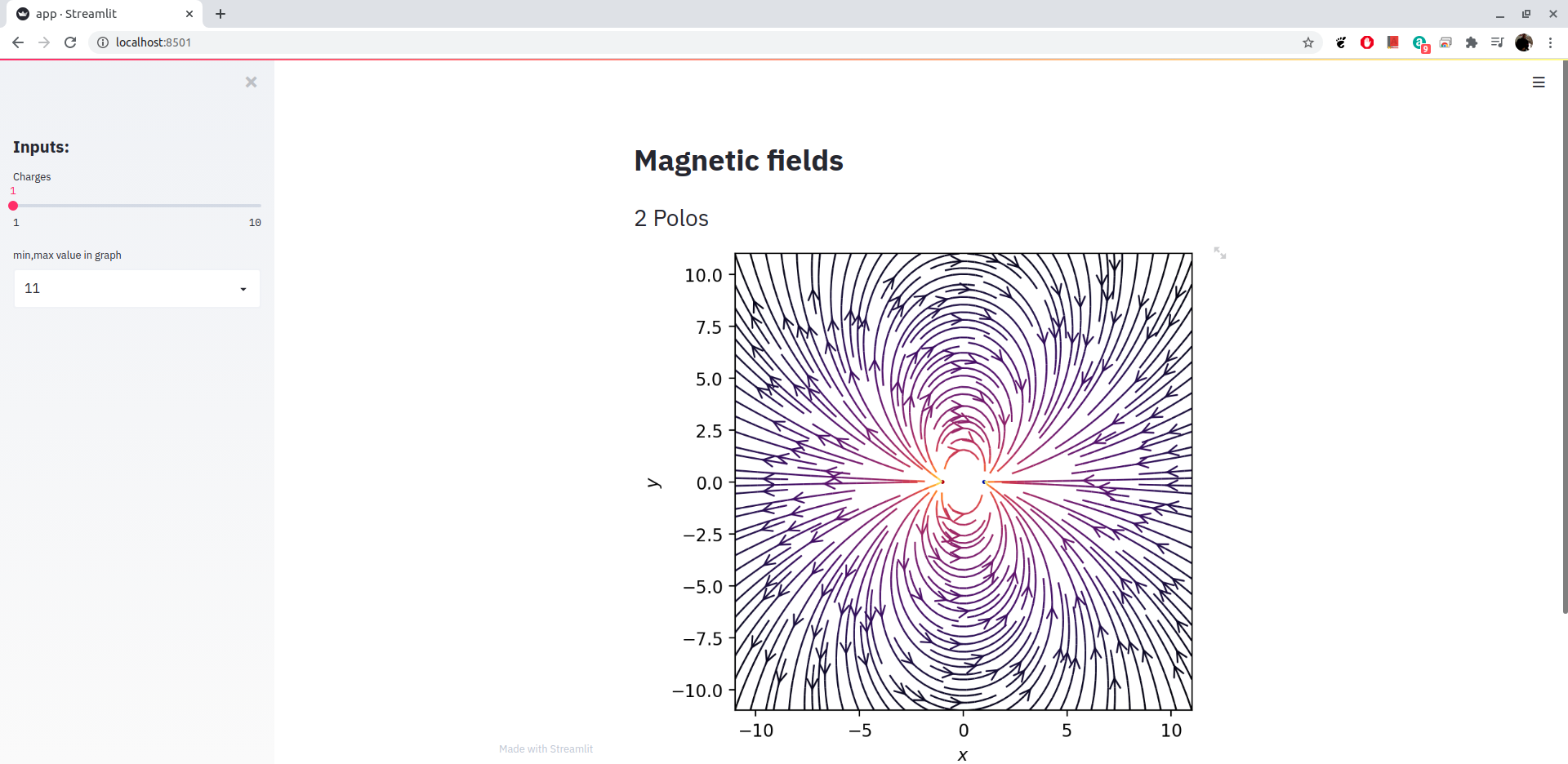
You get the following image of the startup:

Image of the page:

You can see a demonstration of its use in the video on youtube:

A future article will show in detail the different html components that Streamlit has.

You can find the repository with the code for the article on github

Make a donation! If you liked the article you can make a donation with Bitcoin (BTC) using the digital wallet of your choice to the following address: 17MtNybhdkA9GV3UNS6BTwPcuhjXoPrSzV

Or by scanning the QR code from your wallet: