This article is based on an English article from the scipython blog, called Visualizing a vector field with matplotlib.

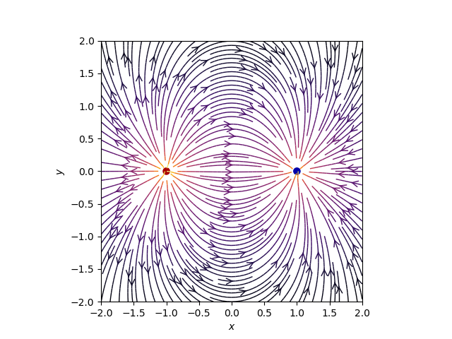
Matplotlib provides a function called streamplot, to create streamlines that can be used to represent vector fields. The python code shows the representation of an electric field from multiple charges. The multiple charges are selected as a power of 2 (1 dipole, 2 quadrupole, etc).

There is a count variable which defines the number of charges; in the first case it is 1 (dipole).

The code is shown below:

#!/usr/bin/env python3

# coding: utf-8


# # Se importan los módulos necesarios para la graficación

import numpy as np

import matplotlib.pyplot as plt

from matplotlib.patches import Circle



# # Función que retorna el campo Eléctrico.

def E(q, r0, x, y):

    """Retorna el vector de campo eléctrico E=(Ex,Ey) de una carga q en r0"""

    den = np.hypot(x-r0[0], y-r0[1])**3

    return q * (x - r0[0]) / den, q * (y - r0[1]) / den



# # puntos de los ejes x e y.

nx, ny = 64, 64

x = np.linspace(-2, 2, nx)

y = np.linspace(-2, 2, ny)

X, Y = np.meshgrid(x, y)



# # Crear un multipolo con nq cargas

# count = número de q. En ese caso es 1 dipolo

count = 1

nq = 2**int(count)

charges = []

for i in range(nq):

    q = i%2 * 2 - 1

    charges.append((q, (np.cos(2*np.pi*i/nq), np.sin(2*np.pi*i/nq))))



# # Vector de campo eléctrico como componentes separados (Ex,Ey)

Ex, Ey = np.zeros((ny, nx)), np.zeros((ny, nx))

for charge in charges:

    ex, ey = E(*charge, x=X, y=Y)

    Ex += ex

    Ey += ey



fig = plt.figure()

ax = fig.add_subplot(111)





# # Dibujar las líneas de flujo con mapa de colores y estilos apropiados.

color = 2 * np.log(np.hypot(Ex, Ey))

ax.streamplot(x, y, Ex, Ey, color=color, linewidth=1, cmap=plt.cm.inferno,

              density=2, arrowstyle='->', arrowsize=1.5)





# # Agregar circulos para las cargas.

charge_colors = {True: '#aa0000', False: '#0000aa'}

for q, pos in charges:

    ax.add_artist(Circle(pos, 0.05, color=charge_colors[q>0]))





# # Graficar

ax.set_xlabel('$x$')

ax.set_ylabel('$y$')

ax.set_xlim(-2,2)

ax.set_ylim(-2,2)

ax.set_aspect('equal')

plt.show()

When the code is run you get the following plot:

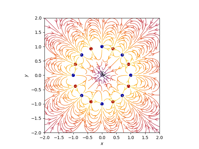
The next plot is with count set to 4, that is 8 poles:

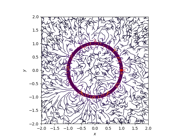
And the last plot is with count at 10, that is 20 poles:

You can get the python code and the jupyter notebook from a github repository.

Make a donation! If you liked the article you can make a donation with Bitcoin (BTC) using the digital wallet of your choice to the following address: 17MtNybhdkA9GV3UNS6BTwPcuhjXoPrSzV

Or by scanning the QR code from your wallet: