After a while without writing, I am resuming the Data Science articles, this time with data visualization. For this we will use the statistics from a data repository about pokemon.
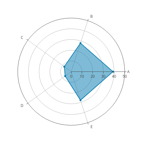
The radar chart is a chart that consists of a sequence of equi-angular spokes, called radii, with each spoke representing one of the variables. The length of a spoke is proportional to the magnitude of the variable for the data point relative to the maximum magnitude of the variable across all data points. A line is drawn connecting the data values for each spoke. This gives the plot a star-like appearance (wikipedia). You can see an example in the following figure:
The idea is to show multiple variables from the information we have about the pokemons. The data repository where the data to work with comes from is the kaggle (broken link) site.
The Python library used in this article to visualize the data with the radar chart is called plotly; at the following link you can see a gallery of charts using python, since this library can also be used with the R Language and Javascript. The good thing about plotly is that it adds more interactivity or dynamism to the charts; they are not simple static charts. Plotly can be used online or offline.
The idea for this article about visualizing pokemon statistics using plotly came from an article where they use the radar chart but with matplotlib.
You can see the basic tutorial on how to use the radar chart in plotly at the following link.
This article is based on a notebook found on kaggle (broken link).
The information the repository contains is the following:
- #: ID of each pokemon.
- Name: Name of each pokemon.
- Type 1: Each pokemon has a type, which determines its weakness/resistance to attacks.
- Type 2: Some pokemon have two types.
- Total: Sum of all the stats.
- HP: Hit point, or health.
- Defense: Level of resistance to attacks.
- SP Atk: special attack.
- SP Def: Resistance against special attacks.
- Speed: Attack speed.
Visualizing pokemon statistics using a radar chart
####Links of interest
- https://typewind.github.io/2017/09/29/radar-chart/
- https://www.kaggle.com/abcsds/pokemon/data (broken link)
- https://plot.ly/python/radar-chart/
- https://www.kaggle.com/thebrownviking20/intermediate-visualization-tutorial-using-plotly (broken link)
Import the necessary libraries
In [1]:
import pandas as pd
import numpy as np
import plotly.plotly as py
import plotly.graph_objs as go
import plotly

import matplotlib.pyplot as plt
from plotly import tools
from plotly.offline import init_notebook_mode, iplot
init_notebook_mode(connected=True)
import plotly.figure_factory as ff
from IPython.display import HTML, Image
Se lee y convierte el archivo csv de los datos de pokemon en un dataframe
In [2]:
df=pd.read_csv("./datos/Pokemon.csv")
Se muestra las 5 primeras filas de datos
In [3]:
df.head()Out[3]:
| # | Name | Type 1 | Type 2 | Total | HP | Attack | Defense | Sp. Atk | Sp. Def | Speed | Generation | Legendary | |
|---|---|---|---|---|---|---|---|---|---|---|---|---|---|
| 0 | 1 | Bulbasaur | Grass | Poison | 318 | 45 | 49 | 49 | 65 | 65 | 45 | 1 | False |
| 1 | 2 | Ivysaur | Grass | Poison | 405 | 60 | 62 | 63 | 80 | 80 | 60 | 1 | False |
| 2 | 3 | Venusaur | Grass | Poison | 525 | 80 | 82 | 83 | 100 | 100 | 80 | 1 | False |
| 3 | 3 | VenusaurMega Venusaur | Grass | Poison | 625 | 80 | 100 | 123 | 122 | 120 | 80 | 1 | False |
| 4 | 4 | Charmander | Fire | NaN | 309 | 39 | 52 | 43 | 60 | 50 | 65 | 1 | False |
The data type of each column in the dataframe is shown.
In [4]:
df.info()
<class 'pandas.core.frame.DataFrame'>
RangeIndex: 800 entries, 0 to 799
Data columns (total 13 columns):
#             800 non-null int64
Name          800 non-null object
Type 1        800 non-null object
Type 2        414 non-null object
Total         800 non-null int64
HP            800 non-null int64
Attack        800 non-null int64
Defense       800 non-null int64
Sp. Atk       800 non-null int64
Sp. Def       800 non-null int64
Speed         800 non-null int64
Generation    800 non-null int64
Legendary     800 non-null bool
dtypes: bool(1), int64(9), object(3)
memory usage: 75.9+ KB
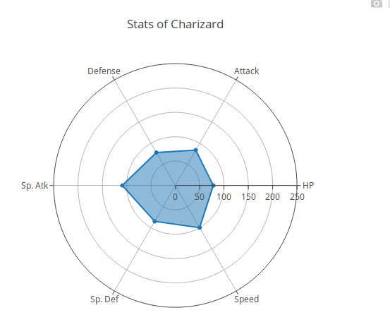
Visualizing the data of a single pokemon In [5]:
#Se busca los datos del pokemon Charizard
x = df[df["Name"] == "Charizard"]
#Se crea la grafica scatterpolar donde se le pasa las variables que se quiere graficar. HP, Ataque, defensa, SP atk,
#Sp def, velocidad y se define los nombres de los ejes.
data = [go.Scatterpolar(
r = [x['HP'].values[0],x['Attack'].values[0],x['Defense'].values[0],x['Sp. Atk'].values[0],x['Sp. Def'].values[0],x['Speed'].values[0],x["HP"].values[0]],
theta = ['HP','Attack','Defense','Sp. Atk','Sp. Def','Speed','HP'],
fill = 'toself'
)]
# se crea el layout, donde se le pasa un diccionario donde se define los ejes de los radios, que son visibles y
#su rango en este caso desde 0 a 250, no se muestra legenda, y el título de la gráfica.
layout = go.Layout(
polar = dict(
radialaxis = dict(
visible = True,
range = [0, 250]
)
),
showlegend = False,
title = "Stats of {}".format(x.Name.values[0])
)
#Se crea la instancia fig donde se pasa los datos y el layout.
fig = go.Figure(data=data, layout=layout)
#Se gràfica la gráfica
iplot(fig, filename = "Single Pokemon stats")
Comparing 2 pokemons In [6]:
# Se crea una función donde se hace la comparación vía gráfica de la estadística de dos pokemons.
def compare2pokemon(x,y):
    #Se  captura los datos de los dos pokemons
    x = df[df["Name"] == x]
    y = df[df["Name"] == y]

    #Se define lo que se quiere gráficar del primer y segundo pokemon.
    trace0 = go.Scatterpolar(
      r = [x['HP'].values[0],x['Attack'].values[0],x['Defense'].values[0],x['Sp. Atk'].values[0],x['Sp. Def'].values[0],x['Speed'].values[0],x["HP"].values[0]],
      theta = ['HP','Attack','Defense','Sp. Atk','Sp. Def','Speed','HP'],
      fill = 'toself',
      name = x.Name.values[0]
    )

    trace1 = go.Scatterpolar(
      r = [y['HP'].values[0],y['Attack'].values[0],y['Defense'].values[0],y['Sp. Atk'].values[0],y['Sp. Def'].values[0],y['Speed'].values[0],y["HP"].values[0]],
      theta = ['HP','Attack','Defense','Sp. Atk','Sp. Def','Speed','HP'],
      fill = 'toself',
      name = y.Name.values[0]
    )

    #se define data como una lista que contiene los datos de los dos pokemon
    data = [trace0, trace1]

    #Se define el layout como en la gráfica anterior.
    layout = go.Layout(
      polar = dict(
        radialaxis = dict(
          visible = True,
          range = [0, 200]
        )
      ),
      showlegend = True,
      title = "{} vs {}".format(x.Name.values[0],y.Name.values[0])
    )
    #Se crea la instancia donde se pasa los datos y el layout
    fig = go.Figure(data=data, layout=layout)
    #Se crea la grafica.
    iplot(fig, filename = "Two Pokemon stats")
In [7]:
# Se compara primeape y muk
compare2pokemon("Primeape", "Muk")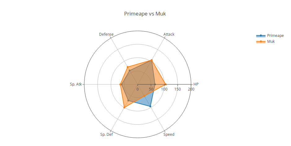
Later articles will keep showing examples of using the plotly chart gallery.
Make a donation! If you liked the article you can make a donation with Bitcoin (BTC) using the digital wallet of your choice to the following address: 17MtNybhdkA9GV3UNS6BTwPcuhjXoPrSzV
Or by scanning the QR code from your wallet: