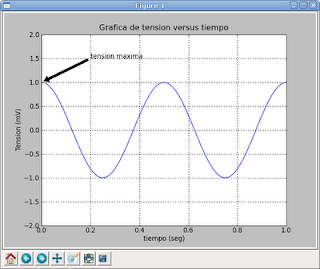
In the following example we will plot a sinusoidal curve over a defined time range.
>>> import numpy
>>> import pylab
>>> t = numpy.arange(0.0, 1.0+0.01, 0.01)
>>> s = numpy.cos(2*2*numpy.pi*t)
>>> pylab.plot(t, s)
[]
>>> pylab.xlabel('tiempo (seg)')
>>> pylab.ylabel('Tension (mV)')
>>> pylab.title('Grafica de tension versus tiempo')
>>> pylab.axis([0,1, -2,2])
>>> pylab.grid(True)
>>> pylab.annotate('tension maxima', xy=(0, 1), xytext=(0.2, 1.5),arrowprops=dict(facecolor='black', shrink=0.05),)

>>> pylab.savefig('grafica.png')
>>> pylab.show()
The numpy and pylab modules are imported, then the time axis range is defined with a numpy function, then the voltage axis is defined with the cosine function, both time and voltage are plotted, both axes are labeled, a title is set for the plot, the axes limits are defined, a grid is defined, and an annotation is defined, setting the annotation text, then the position of the arrow, the position of the text and the characteristics of the arrow; the plot is saved and displayed.
===
Make a donation! If you liked the article you can make a donation with Bitcoin (BTC) using the digital wallet of your choice to the following address: 17MtNybhdkA9GV3UNS6BTwPcuhjXoPrSzV
Or by scanning the QR code from your wallet: