The theorem proves that exact reconstruction of a continuous periodic baseband signal from its samples is mathematically possible if the signal is band-limited and the sampling rate is greater than twice its bandwidth. The article will show sampling at different frequencies, from double the base frequency down to a lower value.
A bit more theory: According to the sampling theorem, a continuous signal x (t) band-limited to B Hz can be recovered from its samples x [n] = x (n * T), where n is an integer, if T is less than or equal to 1 / (2B), without losing any information. And we call 2B the Nyquist rate.
Sampling at a rate lower than the Nyquist rate is called undersampling, and the aliasing effect occurs.
If you want more information about the Sampling Theorem you can check wikipedia.
This article is based on an article in English "The sampling theorem explained with numpy".
The code is shown below:
#!/usr/bin/env python

#De numpy se importa lo necesario para graficar la

#funcion seno

from numpy import linspace,sin,cos,pi,ceil,floor,arange

#De pylab se importa plot, show y axis. Lo necesario para crear

#la grafica

from pylab import plot,show,axis

#Muestreo de una seganl de ancho de banda 40 hz

# con velocidad de muestreo de 80 Hz

f = 40;  # Hz

#Tiempo minimo y maximo

tmin = -0.3;

tmax = 0.3;

#Se define el tiempo de la segnal.

t = linspace(tmin, tmax, 400);

#Se define la segnal de muestreo

x = cos(2*pi*t) + cos(2*pi*f*t)

#Se grafica el tiempo y la segnal.

plot(t, x)

# sampling the signal with a sampling rate of 80 Hz

# in this case, we are using the Nyquist rate.

#Muestreo de la segnal con una velocidad de muestreo de 80 Hz.

#Periodo de muestreo

T = 1/80.0;

#Tiempo minimo

nmin = ceil(tmin / T);

#Tiempo maximo

nmax = floor(tmax / T);

#Tiempo de la segnal.

n = arange(nmin,nmax);

#Segnal a la velocidad de muestreo

x1 = cos(2*pi*n*T) + cos(2*pi*f*n*T);

#Se grafica la segnal.

plot(n*T, x1, 'bo')

#Muestreo de la segnal con una velocidad de muestreo de 35Hz.

#Note que 35Hz esta por debajo de la velocidad de Nyquist.

T = 1/35.0;

nmin = ceil(tmin / T);

nmax = floor(tmax / T);

n = arange(nmin,nmax);

x2 = cos(2*pi*n*T) + cos(2*pi*f*n*T);

plot(n*T, x2, '-r.',markersize=15)

axis([-0.3, 0.3, -1.5, 2.3])

show()
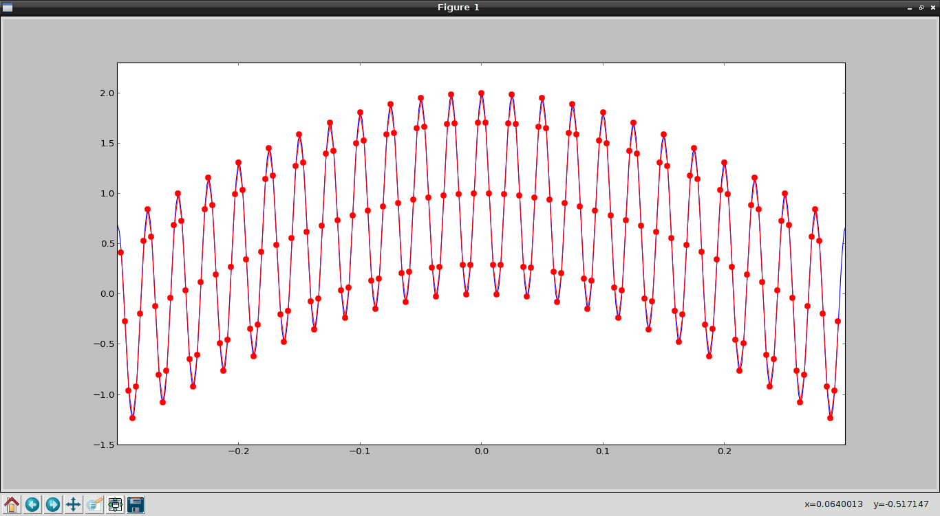
The generated plot is the following:
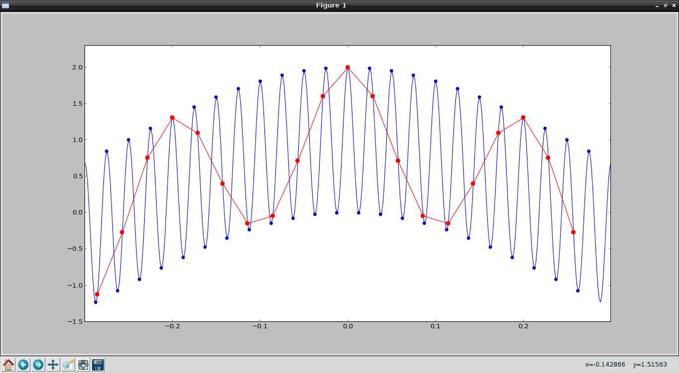
The blue dots are the sampling at 80Hz and the red dots are the sampling at 35 Hz; note that sampling at 80 Hz is enough to capture the oscillation of the signal.
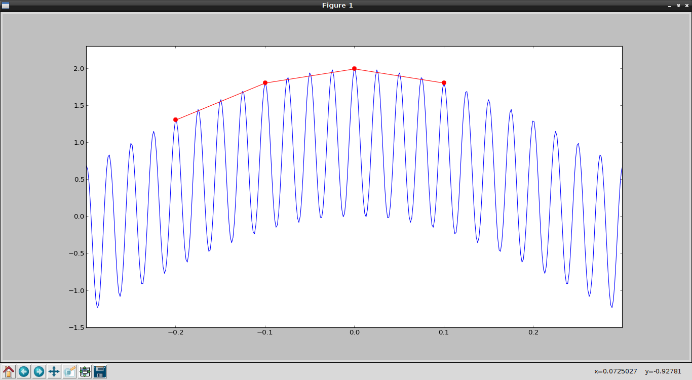
The following plot has a sampling at 10 Hz, which is below the base frequency of the signal (40 Hz).
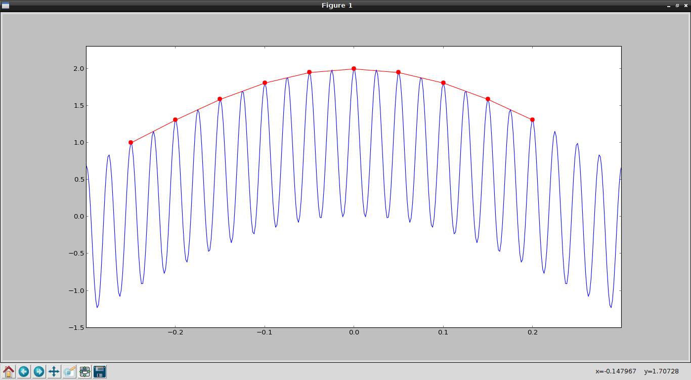
Now the sampling frequency at 20 Hz is shown:
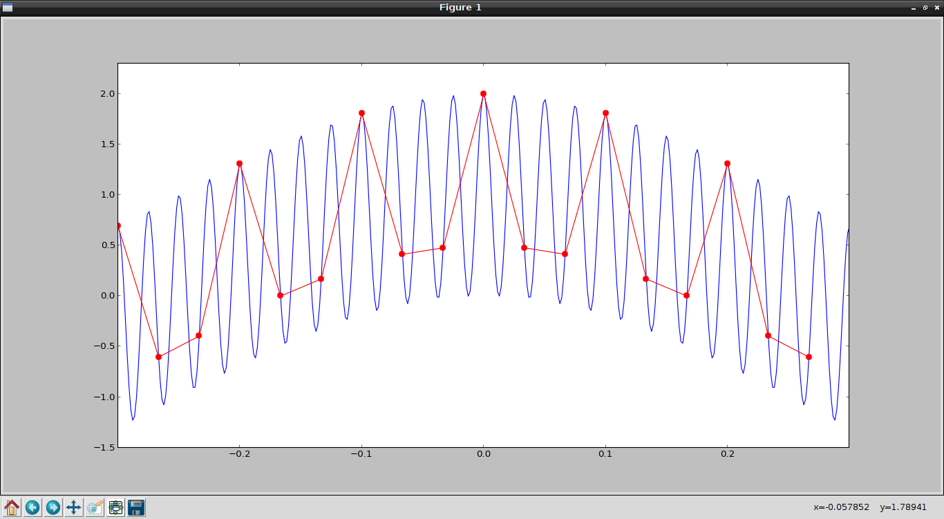
Next, the sampling frequency at 30 Hz is shown:
Finally, the plot at a sampling frequency of 320 Hz is shown:
As can be seen, the lower the sampling frequency relative to the base frequency of the signal, the less the original signal can be generated from the sample; as the sampling frequency increases up to the base frequency, there are more samples for the recovery but it is still not enough; it is from double the base frequency onward that the signal can be reconstructed from the samples.
Make a donation! If you liked the article you can make a donation with Bitcoin (BTC) using the digital wallet of your choice to the following address: 17MtNybhdkA9GV3UNS6BTwPcuhjXoPrSzV
Or by scanning the QR code from your wallet: