While going through some scripts on my machine I found one that calculates the physics of a vertical launch.
The precision of the calculation is achieved with an array that defines the values of the time variable.
This is possible thanks to the numpy module, which lets you create an array of decimal values with specific steps between each element of the array.
If you need an array with values from 0 to 5.6 with steps of 0.1, run the following instruction:
#!/usr/bin/env python2.6
# -*- coding: utf-8 -*-
import numpy as np
arreglo = np.arange(0, 5.60,0.1)
print arreglo
[ 0.   0.1  0.2  0.3  0.4  0.5  0.6  0.7  0.8  0.9  1.   1.1  1.2  1.3  1.4
  1.5  1.6  1.7  1.8  1.9  2.   2.1  2.2  2.3  2.4  2.5  2.6  2.7  2.8  2.9
  3.   3.1  3.2  3.3  3.4  3.5  3.6  3.7  3.8  3.9  4.   4.1  4.2  4.3  4.4
  4.5  4.6  4.7  4.8  4.9  5.   5.1  5.2  5.3  5.4  5.5]
There are 2 functions, fx(t) and fy(t), both of which calculate the position of a body in a vertical launch. We calculate the time the body takes to fall to the floor from a height of 100 m with an initial velocity in X and Y, and the acceleration on the X axis and gravity.
I simply use matplotlib to generate the plot; in an upcoming article I will show how to use glade+python+gtk with matplotlib to get the two plots shown in the following figure:
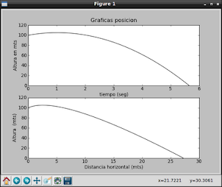
The first plot shows the body's trajectory in terms of its height versus the time it takes to fall. The second plot shows the trajectory in terms of height and horizontal distance; it would be a description of the path of the body's launch.
The code that performs the calculation and draws the plots is shown below:
#!/usr/bin/env python
# -*- coding: utf-8 -*-

#Se importa el modulo numpy para generar un arreglo con los datos de la variable tiempo
import numpy as np
#Se importa matplotlib para generar la grafica.
import matplotlib.pyplot as plt


#Se define la funcion x(t) de la ecuacion de posicion (movimiento horizontal)
def fx (t):
    #Se define la posicion inicial en 0
    x0 = 0
    #Se define la velocidad inicial en 2 mts/seg
    v0x = 2
    #Se define la aceleracion en 1 mts/seg^2
    ax = 1
    #Se hace el calculo de la posicion con respecto al tiempo
    x = x0 + v0x*t + 0.5*ax*t**2
    return x

#Se define la funcion y(t) de la ecuacion de posicion altura
def fy(t):
    #Se define la altura inicial en 100 mts
    y0 = 100
    #Se define la velocidad inicial en 10 mts/seg
    v0y = 10
    #Se define la gravedad en 9.81 mts/seg^2
    g = 9.81
    #Se realiza el calculo de l posicion en funcion del tiempo
    y = y0 + v0y*t - 0.5*g*t**2
    return y


#Programa principal
def main():
    #Se define un range desde 0 a 5.65 con intervalos de 0.01.
    tiempo = np.arange(0, 5.65,0.01)
    #Se define la figura
    plt.figure(1)
    #Se define la grafica.
    plt.subplot(211)
    #Se despligega la grafica de la distancia en X en funcion del tiempo
    plt.plot(tiempo, fy(tiempo),"k")
    #Se Coloca un titulo a la grafica y la informacion del eje y (tiempo)
    plt.title("Graficas posicion")
    plt.xlabel("tiempo (seg)")
    plt.ylabel("Altura en mts")
    #Se muestra la grafica de posicion en X respecto a la altura.
    plt.subplot(212)
    #Se grafica la funcion fx vs fy
    plt.plot(fx(tiempo),fy(tiempo),'k')
    #Se muestra la info del eje X y Y
    plt.xlabel("Distancia horizontal (mts)")
    plt.ylabel("Altura  (mts)")
    #Se muestra las graficas.
    plt.show()


if __name__ == "__main__":
    main()
As I mentioned before, in a following article I will show this same example but using glade.
===
Make a donation! If you liked the article you can make a donation in Bitcoin (BTC) using the digital wallet of your choice to the following address: 17MtNybhdkA9GV3UNS6BTwPcuhjXoPrSzV
Or by scanning the QR code from your wallet: