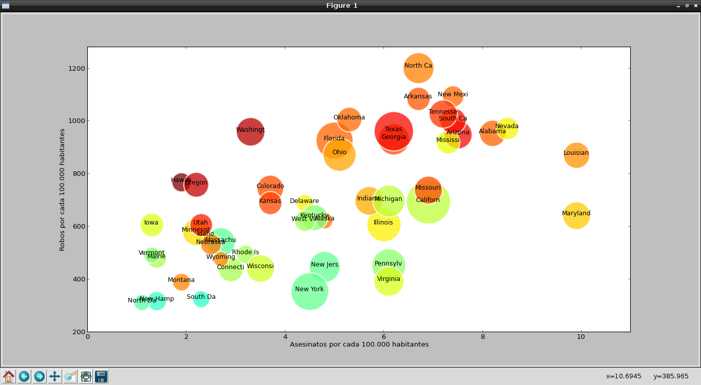
Bubble charts present data as a series of bubbles whose size is proportional to the amount of data.
A chart of this type is very effective for showing the number of products sold in a certain region.
There is a tool called Trendalyzer, developed by the Gapminder Foundation, which turns statistical series into interactive charts.
Hans Rosling, one of the founders of Gapminder, is the one who has shown the potential of the tool. The following video is a demonstration of the tool:
With matplotlib in Python you can also create bubble charts; this article is based on an English article called "How to make Bubble charts with matplotlib ".
The data will be taken from a csv file; it is crime statistics in the United States by state for the year 2005. The csv file can be downloaded here.
The information in the csv file looks like this (the first lines of the file are shown):
state,murder,forcible_rape,robbery,aggravated_assault,burglary,larceny_theft,motor_vehicle_theft,population
United States,5.6,31.7,140.7,291.1,726.7,2286.3,416.7,295753151
Alabama,8.2,34.3,141.4,247.8,953.8,2650,288.3,4545049
Alaska,4.8,81.1,80.9,465.1,622.5,2599.1,391,669488
Arizona,7.5,33.8,144.4,327.4,948.4,2965.2,924.4,5974834
Arkansas,6.7,42.9,91.1,386.8,1084.6,2711.2,262.1,2776221
California,6.9,26,176.1,317.3,693.3,1916.5,712.8,35795255
As you can see, the first line has the title of each column, the second line has the total for the United States, and then the information by state is shown.
For programming purposes the first and second lines are not relevant for the bubble chart.
Here is the program code:
#!/usr/bin/env python
# -*- coding: utf-8 -*-

from pylab import *
from scipy import *

#Leer los datos desde el archivo csv
#Archivo original
#durl = 'http://datasets.flowingdata.com/crimeRatesByState2005.csv'
#Archivo modificado.
durl = 'http://127.0.0.1/descargas/crimeRatesByState2005-es.csv'
#Se captura los datos del archivo csv.
rdata = genfromtxt(durl,dtype='S8,f,f,f,f,f,f,f,i',delimiter=',')

rdata[0] = zeros(8) # se elimina los titulos
rdata[1] = zeros(8) # se elimina la estadistica total de estados unidos (2da linea)
x = []
y = []
color = []
area = []

#Se captura los datos de cada fila
for data in rdata:
    x.append(data[1]) # asesinatos
    y.append(data[5]) # robo
    color.append(data[6]) # hurtos
    area.append(sqrt(data[8])) # poblacion
    # graficando las primeras 8 letras del nombre del estado
    text(data[1], data[5],data[0],size=11,horizontalalignment='center')


# se crea la grafica
sct = scatter(x, y, c=color, s=area, linewidths=2, edgecolor='w')
sct.set_alpha(0.75)
#Se define los ejes
axis([0,11,200,1280])
#Las etiquetas de cada eje
xlabel('Asesinatos por cada 100.000 habitantes')
ylabel('Robos por cada 100.000 habitantes')
show()
The following figure shows the result of running the program:
Make a donation! If you liked the article you can make a donation with Bitcoin (BTC) using the digital wallet of your choice to the following address: 17MtNybhdkA9GV3UNS6BTwPcuhjXoPrSzV
Or by scanning the QR code from your wallet: