Blog | Analyzing climate change data and atmospheric CO2 levels with Python and pandas.

Continuing with the articles about data science, this time data on global and per-country climate information, as well as CO2 levels, will be analyzed.

I found this data and project on the kaggle (broken link) site, which is a site for publishing data science projects. You can find the data for this article at the following link (broken link).

The code in this article is based on the article on kaggle on the subject, in English: Climate Change and CO2 levels in atmosphere (broken link).

This article explores the global changes in mean temperature and the increase in the concentration of CO2 in the atmosphere.

The data comes from the following files:

GlobalLandTemperaturesByCountry.csv: Contains the temperature information by country.
GlobalTemperatures.csv: Contains the global temperature information.
archive.csv: Contains the information on CO2 levels in the atmosphere.

The notebook is shown below:

https://www.kaggle.com/derevirn/data-analysis-on-climate-change/notebook (broken link) https://www.kaggle.com/derevirn/data-analysis-on-climate-change/data (broken link)

Import the pandas, matplotlib and seaborn libraries.

In [1]:

import pandas as pd
import matplotlib.pyplot as plt
import seaborn as sns

Create the dataframes from the csv files.

In [2]:

# Se crea el dataframe data_pais, data_vzla, data_global y co2_ppm

data_pais = pd.read_csv("./datos/GlobalLandTemperaturesByCountry.csv")
#Se crea una copia del dataframe obteniendo solo la información de Venezuela.
data_vzla = data_pais[data_pais["Country"] == "Venezuela"].copy()
data_vzla["dt"] = pd.to_datetime(data_vzla["dt"])

#Se crea una copia del dataframe obteniendo solo la información de Argentina.
data_arg = data_pais[data_pais["Country"] == "Argentina"].copy()
data_arg["dt"] = pd.to_datetime(data_arg["dt"])

#Se crea una copia del dataframe obteniendo solo la información de USA.
data_canada = data_pais[data_pais["Country"] == "Canada"].copy()
data_canada["dt"] = pd.to_datetime(data_canada["dt"])

#Se crea una copia del dataframe obteniendo solo la información de Mexico.
data_mexico = data_pais[data_pais["Country"] == "Mexico"].copy()
data_mexico["dt"] = pd.to_datetime(data_mexico["dt"])

#Se crea una copia del dataframe obteniendo solo la información de Brasil.
data_brasil = data_pais[data_pais["Country"] == "Brazil"].copy()
data_brasil["dt"] = pd.to_datetime(data_brasil["dt"])

#Se crea una copia del dataframe obteniendo solo la información de Venezuela.
data_chile = data_pais[data_pais["Country"] == "Chile"].copy()
data_chile["dt"] = pd.to_datetime(data_chile["dt"])

#Se crea el dataframe de la temperatura global. 
data_global = pd.read_csv("./datos/GlobalTemperatures.csv")
#Se modifica la fecha y hora como datetime.
data_global["dt"] = pd.to_datetime(data_global["dt"])
#Se crea el dataframe del co2.
co2_ppm = pd.read_csv("./datos/archive.csv")

The dataframes created.

In [3]:

data_pais.head()

Out[3]:

ID	dt	Average Temperature	Average Temperature Uncertainty	Country
0	1743-11-01	4.384	2.294	Åland
1	1743-12-01	NaN	NaN	Åland
2	1744-01-01	NaN	NaN	Åland
3	1744-02-01	NaN	NaN	Åland
4	1744-03-01	NaN	NaN	Åland

As can be seen, there is the date, the average temperature, the average temperature uncertainty and the country. In [4]:

data_pais.info()
<class 'pandas.core.frame.DataFrame'>
RangeIndex: 577462 entries, 0 to 577461
Data columns (total 4 columns):
dt                               577462 non-null object
AverageTemperature               544811 non-null float64
AverageTemperatureUncertainty    545550 non-null float64
Country                          577462 non-null object
dtypes: float64(2), object(2)
memory usage: 17.6+ MB

The data types of the columns are: dt is object, average temperature and average temperature uncertainty are float64, and country is object

Venezuela

In [5]:

data_vzla.head()

Out[5]:

ID	dt	Average Temperature	Average Temperature Uncertainty	Country
562339	1824-01-01	24.613	0.824	Venezuela
562340	1824-02-01	24.670	2.017	Venezuela
562341	1824-03-01	25.527	1.065	Venezuela
562342	1824-04-01	25.732	1.771	Venezuela
562343	1824-05-01	24.999	1.157	Venezuela

This is the same information as above but only for Venezuela. In [6]:

data_vzla.describe().T

Out[6]:

	count	mean	std	min	25%	50%	75%	max
AverageTemperature	2086.0	25.025686	0.703189	22.777	24.52325	24.9825	25.49525	27.807
AverageTemperatureUncertainty	2086.0	0.586000	0.398460	0.084	0.31000	0.4540	0.76000	4.120

There are 2086 data points, for which the average temperature is 25.025 degrees and the uncertainty is 0.586; the standard deviation of the average temperature is 0.703 and of the uncertainty is 0.398; the minimum temperature was 22.77 and the maximum 27.807. In [7]:

data_vzla.corr()

Out[7]:

| | AverageTemperature | AverageTemperatureUncertainty | |:--------------------------- - | :---------------: | :---------------------------: | |AverageTemperature | 1.000000 | -0.319882 | |AverageTemperatureUncertainty | -0.319882 | 1.000000 |

The two variables are, to a certain extent, inversely correlated. Argentina In [8]:

data_arg.head()

Out[8]:

ID	dt	Average Temperature	Average Temperature Uncertainty	Country
25466	1855-05-01	10.745	1.499	Argentina
25467	1855-06-01	6.995	2.073	Argentina
25468	1855-07-01	6.901	1.568	Argentina
25469	1855-08-01	9.097	1.412	Argentina
25470	1855-09-01	11.316	1.384	Argentina

In [9]:

data_arg.describe().T

Out[9]:

	count	mean	std	min	25%	50%	75%	max
AverageTemperature	1900.0	14.621194	4.846885	4.796	10.13225	14.6305	19.27875	23.290
AverageTemperatureUncertainty	1900.0	0.527338	0.465652	0.083	0.20900	0.3035	0.74525	2.974

Brazil

In [10]:

data_brasil.head()

Out[10]:

ID	dt	Average Temperature	Average Temperature Uncertainty	Country
77110	1832-01-01	24.935	1.372	Brazil
77111	1832-02-01	24.505	1.953	Brazil
77112	1832-03-01	24.617	1.359	Brazil
77113	1832-04-01	23.990	2.013	Brazil
77114	1832-05-01	23.124	1.592	Brazil

In [11]:

data_brasil.describe().T

Out[11]:

	count	mean	std	min	25%	50%	75%	max
AverageTemperature	2164.0	24.699256	0.978787	21.797	24.02250	24.8295	25.44975	27.151
AverageTemperatureUncertainty	2164.0	0.572940	0.411794	0.060	0.24375	0.4160	0.84000	3.353

Chile

In [12]:

data_chile.head()

Out[12]:

ID	dt	AverageTemperature	AverageTemperatureUncertainty	Country
108248	1855-05-01	7.152	1.296	Chile
108249	1855-06-01	4.257	1.641	Chile
108250	1855-07-01	4.113	1.313	Chile
108251	1855-08-01	5.508	1.168	Chile
108252	1855-09-01	6.684	1.153	Chile

In [13]:

data_chile.describe().T

Out[13]:

	count	mean	std	min	25%	50%	75%	max
AverageTemperature	1900.0	9.383474	3.179081	3.206	6.502	9.3815	12.37775	15.493
AverageTemperatureUncertainty	1900.0	0.572654	0.418011	0.114	0.281	0.3825	0.80300	2.408

Mexico

In [14]:

data_mexico.head()

Out[14]:

ID	dt	AverageTemperature	AverageTemperatureUncertainty	Country
338438	1835-01-01	15.810	1.484	Mexico
338438	1835-01-01	15.810	1.484	Mexico
338439	1835-02-01	14.911	1.579	Mexico
338440	1835-03-01	16.826	1.858	Mexico
338441	1835-04-01	19.925	1.966	Mexico
338442	1835-05-01	22.037	1.609	Mexico

In [15]:

data_mexico.describe().T

Out[15]:

	count	mean	std	min	25%	50%	75%	max
AverageTemperature	2145.0	20.567558	3.753343	12.064	17.109	21.050	24.164	26.926
AverageTemperatureUncertainty	2145.0	0.638233	0.547605	0.091	0.226	0.398	0.970	3.699

####Canada In [16]:

data_canada.head()

Out[16]:

ID	dt	AverageTemperature	AverageTemperatureUncertainty	Country
97255	1768-09-01	5.257	3.107	Canada
97256	1768-10-01	-3.393	2.981	Canada
97257	1768-11-01	-12.829	3.967	Canada
97258	1768-12-01	-20.582	4.622	Canada
97259	1769-01-01	-24.756	4.722	Canada

In [17]:

data_canada.describe().T

Out[17]:

	count	mean	std	min	25%	50%	75%	max
AverageTemperature	2504.0	-5.216659	12.878074	-28.736	-17.7025	-4.7285	7.41275	14.796
AverageTemperatureUncertainty	2504.0	1.256211	1.046127	0.123	0.2870	0.8980	2.12025	5.275

Note that the variations in the average temperature uncertainty are greater in Brazil, Venezuela, Mexico and Canada, in that order, compared with Chile and Argentina.

Annual increase in the global average temperature

In [18]:

annual_mean_global = data_global.groupby(data_global["dt"].dt.year).mean()
reference_temperature_global = annual_mean_global.loc[1951:1980].mean()["LandAndOceanAverageTemperature"]
annual_mean_global["Anomaly"] = annual_mean_global["LandAndOceanAverageTemperature"] - reference_temperature_global

In [19]:

plt.figure()
plt.style.use("fivethirtyeight")
annual_mean_global.loc[1960:2015]["Anomaly"].plot(figsize = (10,5), grid=True, legend=True)
plt.title("Anomalia anual de la temperatura promedio global")
plt.xlabel('')
plt.ylabel('Anomalia de la temperatura')
plt.show()

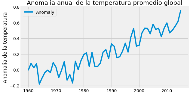
![](/blog/images/analizandodatosdelcambioclimaticoynivelesdeco2enlaatmosferaconpythonypandas-1.png)

Note that the annual temperature increase shows an upward trend that has grown in recent years; this increase in 2015 was 0.75 degrees, which is consistent with climate change.

Venezuela.

The same calculation is done for the case of Venezuela. In [20]:

annual_mean_vzla = data_vzla.groupby(data_vzla["dt"].dt.year).mean()
reference_temperature_vzla = annual_mean_vzla.loc[1951:1980].mean()["AverageTemperature"]
annual_mean_vzla["Anomaly"] = annual_mean_vzla["AverageTemperature"] - reference_temperature_vzla

In [21]:

annual_mean_vzla.head()

Out[21]:

dt	AverageTemperature	AverageTemperatureUncertainty	Anomaly
1824	24.896545	1.516091	-0.420966
1825	25.071583	1.552083	-0.245928
1826	24.871900	1.440800	-0.445611
1827	25.156273	1.474182	-0.161238
1828	24.751818	1.516727	-0.565693

In [22]:

annual_mean_vzla.tail()

Out[22]:

dt	AverageTemperature	AverageTemperatureUncertainty	Anomaly
2009	26.084917	0.353917	0.767406
2010	26.150250	0.341333	0.832739
2011	25.677333	0.336750	0.359822
2012	25.688583	0.401417	0.371072
2013	25.912875	0.484500	0.595364

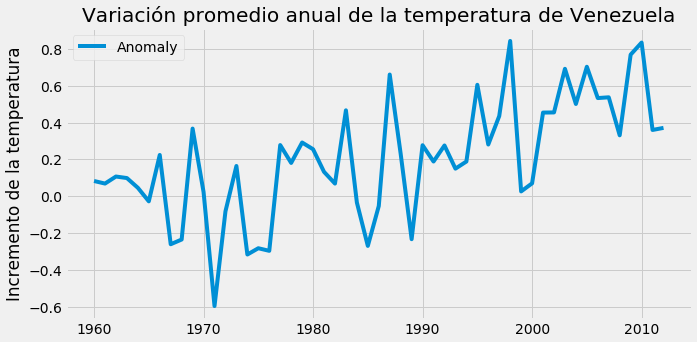
The last record is from 2013, when the increase was 0.595 degrees; there was a peak in 2010 of 0.8332 degrees. In [23]:

plt.figure()
plt.style.use("fivethirtyeight")
annual_mean_vzla.loc[1960:2012]["Anomaly"].plot(figsize = (10,5), grid=True, legend=True)
plt.title("Variación promedio anual de la temperatura de Venezuela")
plt.xlabel('')
plt.ylabel('Incremento de la temperatura')
plt.show()

![](/blog/images/analizandodatosdelcambioclimaticoynivelesdeco2enlaatmosferaconpythonypandas-2.png)

Argentina

In [24]:

annual_mean_arg = data_arg.groupby(data_arg["dt"].dt.year).mean()
reference_temperature_arg = annual_mean_arg.loc[1951:1980].mean()["AverageTemperature"]
annual_mean_arg["Anomaly"] = annual_mean_arg["AverageTemperature"] - reference_temperature_arg

In [25]:

annual_mean_arg.head()

Out[25]:

dt	AverageTemperature	AverageTemperatureUncertainty	Anomaly
1855	11.729250	1.711875	-3.090742
1856	13.998750	1.553167	-0.821242
1857	14.221083	1.993417	-0.598908
1858	14.015667	1.770750	-0.804325
1859	14.414583	1.635583	-0.405408

In [26]:

annual_mean_arg.tail()

Out[26]:

dt	AverageTemperature	AverageTemperatureUncertainty	Anomaly
2009	15.534417	0.215750	0.714425
2010	15.078833	0.218917	0.258842
2011	15.339667	0.219833	0.519675
2012	15.689000	0.265750	0.869008
2013	14.457125	0.276500	-0.362867

In [27]:

plt.figure()
plt.style.use("fivethirtyeight")
annual_mean_arg.loc[1960:2012]["Anomaly"].plot(figsize = (10,5), grid=True, legend=True)
plt.title("Variación promedio anual de la temperatura de Argentina")
plt.xlabel('')
plt.ylabel('Incremento de la temperatura')
plt.show()

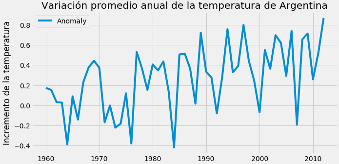
![](/blog/images/analizandodatosdelcambioclimaticoynivelesdeco2enlaatmosferaconpythonypandas-3.png)

In the case of Argentina, the slope of the temperature increase trend is less pronounced.

Brazil

In [28]:

annual_mean_brasil = data_brasil.groupby(data_brasil["dt"].dt.year).mean()
reference_temperature_brasil = annual_mean_brasil.loc[1951:1980].mean()["AverageTemperature"]
annual_mean_brasil["Anomaly"] = annual_mean_brasil["AverageTemperature"] - reference_temperature_brasil

In [29]:

annual_mean_brasil.head()

Out[29]:

dt	AverageTemperature	AverageTemperatureUncertainty	Anomaly
1832	23.858583	1.734500	-1.072247
1833	24.517833	1.450083	-0.412997
1834	24.346750	1.498083	-0.584081
1835	23.537500	1.298583	-1.393331
1836	23.921167	1.426083	-1.009664

In [30]:

annual_mean_brasil.tail()

Out[30]:

dt	AverageTemperature	AverageTemperatureUncertainty	Anomaly
2009	25.600583	0.185667	0.669753
2010	25.812417	0.158000	0.881586
2011	25.428917	0.204833	0.498086
2012	25.717083	0.231000	0.786253
2013	25.348125	0.262250	0.417294

In [31]:

plt.figure()
plt.style.use("fivethirtyeight")
annual_mean_brasil.loc[1960:2012]["Anomaly"].plot(figsize = (10,5), grid=True, legend=True)
plt.title("Variación promedio anual de la temperatura de Brasil")
plt.xlabel('')
plt.ylabel('Incremento de la temperatura')
plt.show()

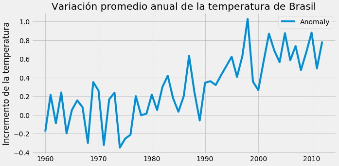
![](/blog/images/analizandodatosdelcambioclimaticoynivelesdeco2enlaatmosferaconpythonypandas-4.png)

In the case of Brazil, a strong increase is noticeable in the 90s with a peak of more than 1 degree, after which the trend has stabilized at 0.79 degrees.

Chile

In [32]:

annual_mean_chile = data_chile.groupby(data_chile["dt"].dt.year).mean()
reference_temperature_chile = annual_mean_chile.loc[1951:1980].mean()["AverageTemperature"]
annual_mean_chile["Anomaly"] = annual_mean_chile["AverageTemperature"] - reference_temperature_chile

In [33]:

annual_mean_chile.head()

Out[33]:

dt	AverageTemperature	AverageTemperatureUncertainty	Anomaly
1855	7.070125	1.424125	-2.510742
1856	8.664083	1.319250	-0.916783
1857	8.645917	1.439250	-0.934950
1858	8.810250	1.428333	-0.770617
1859	9.245583	1.376917	-0.335283

In [34]:

annual_mean_chile.tail()

Out[34]:

dt	AverageTemperature	AverageTemperatureUncertainty	Anomaly
2009	9.994417	0.281917	0.413550
2010	9.712833	0.340000	0.131967
2011	10.032250	0.322250	0.451383
2012	10.272583	0.384583	0.691717
2013	9.877375	0.393875	0.296508

In [35]:

plt.figure()
plt.style.use("fivethirtyeight")
annual_mean_chile.loc[1960:2012]["Anomaly"].plot(figsize = (10,5), grid=True, legend=True)
plt.title("Variación promedio anual de la temperatura de Chile")
plt.xlabel('')
plt.ylabel('Incremento de la temperatura')
plt.show()

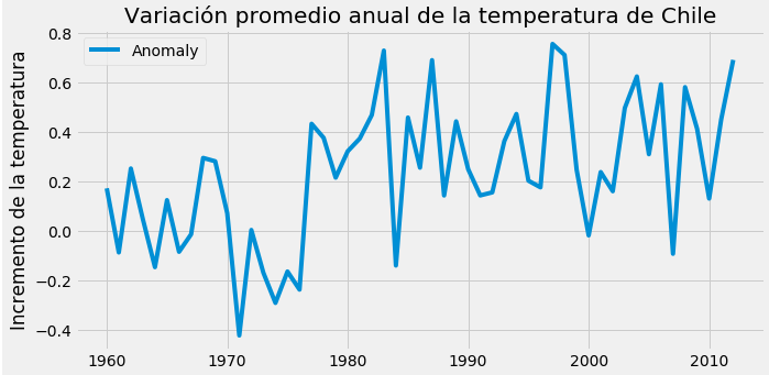
![](/blog/images/analizandodatosdelcambioclimaticoynivelesdeco2enlaatmosferaconpythonypandas-5.png)

The variation does not exceed 0.8 degrees of temperature, with a strong increase between the 70s and 80s and then a peak in the 90s.

Mexico

In [36]:

annual_mean_mexico = data_mexico.groupby(data_mexico["dt"].dt.year).mean()
reference_temperature_mexico = annual_mean_mexico.loc[1951:1980].mean()["AverageTemperature"]
annual_mean_mexico["Anomaly"] = annual_mean_mexico["AverageTemperature"] - reference_temperature_mexico

In [37]:

annual_mean_mexico.head()

Out[37]:

dt	AverageTemperature	AverageTemperatureUncertainty	Anomaly
1835	18.993250	1.684083	-1.745911
1836	19.587167	1.695333	-1.151994
1837	19.671083	1.647667	-1.068078
1838	19.337000	1.862417	-1.402161
1839	19.785833	1.603000	-0.953328

In [38]:

annual_mean_mexico.tail()

Out[38]:

dt	AverageTemperature	AverageTemperatureUncertainty	Anomaly
2009	21.546083	0.205917	0.806922
2010	20.852917	0.217750	0.113756
2011	21.599333	0.245333	0.860172
2012	21.652417	0.324500	0.913256
2013	22.219222	0.365111	1.480061

In [39]:

plt.figure()
plt.style.use("fivethirtyeight")
annual_mean_mexico.loc[1960:2012]["Anomaly"].plot(figsize = (10,5), grid=True, legend=True)
plt.title("Variación promedio anual de la temperatura de Mexico")
plt.xlabel('')
plt.ylabel('Incremento de la temperatura')
plt.show()


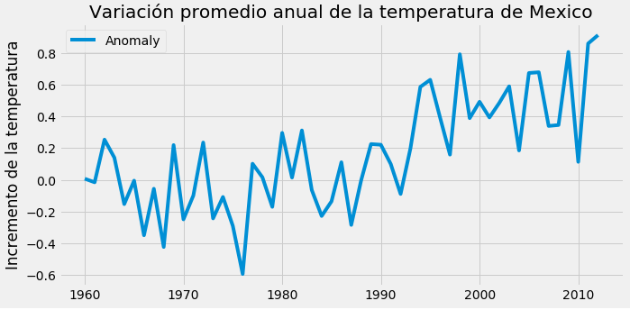
![](/blog/images/analizandodatosdelcambioclimaticoynivelesdeco2enlaatmosferaconpythonypandas-6.png)

Note the upward trend of the temperature in Mexico, reaching 2013 at 1.48 degrees above the average.

####Canada In [40]:

annual_mean_canada = data_canada.groupby(data_canada["dt"].dt.year).mean()
reference_temperature_canada = annual_mean_canada.loc[1951:1980].mean()["AverageTemperature"]
annual_mean_canada["Anomaly"] = annual_mean_canada["AverageTemperature"] - reference_temperature_canada

In [41]:

annual_mean_canada.head()

Out[41]:

dt	AverageTemperature	AverageTemperatureUncertainty	Anomaly
1768	-7.886750	3.66925	-2.969253
1769	-3.427875	3.50550	1.489622
1770	NaN	NaN	NaN
1771	NaN	NaN	NaN
1772	NaN	NaN	NaN

In [42]:

annual_mean_canada.tail()

Out[42]:

dt	AverageTemperature	AverageTemperatureUncertainty	Anomaly
2009	-4.135083	0.231833	0.782414
2010	-1.887917	0.218583	3.029581
2011	-3.557083	0.232583	1.360414
2012	-3.176833	0.300083	1.740664
2013	-1.640667	0.533667	3.276831

In [43]:

plt.figure()
plt.style.use("fivethirtyeight")
annual_mean_canada.loc[1960:2012]["Anomaly"].plot(figsize = (10,5), grid=True, legend=True)
plt.title("Variación promedio anual de la temperatura de Canadá")
plt.xlabel('')
plt.ylabel('Incremento de la temperatura')
plt.show()

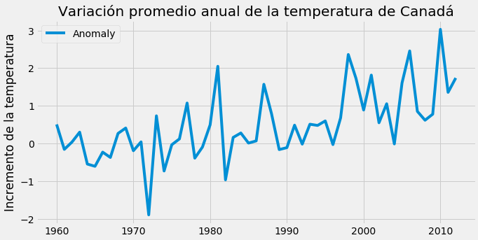
![](/blog/images/analizandodatosdelcambioclimaticoynivelesdeco2enlaatmosferaconpythonypandas-7.png)

Note the upward trend of the temperature in Canada, and the worrying thing is that the variation exceeds 3 degrees in 2013.

Annual CO2 levels in the Atmosphere

In [44]:

plt.figure()
plt.style.use("fivethirtyeight")
annual_co2_ppm = co2_ppm.groupby(co2_ppm["Year"]).mean()
annual_co2_ppm.loc[1960:2015]["Carbon Dioxide (ppm)"].plot(figsize = (10,5), grid=True, legend=True)
plt.title("Nivel anual global de CO2 en la Atmosfera")
plt.ylabel("CO2 partes por millón")
plt.show()

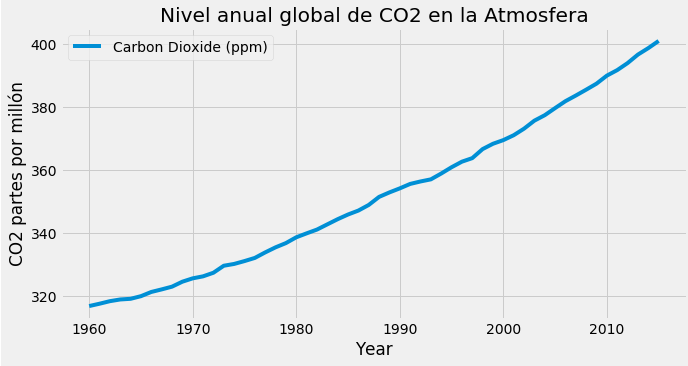
![](/blog/images/analizandodatosdelcambioclimaticoynivelesdeco2enlaatmosferaconpythonypandas-8.png)

Note the annual increase with an upward trend.

The relationship between CO2 and temperature is calculated.

In [45]:

annual_co2_temp = pd.merge(annual_mean_global.loc[1960:2015], annual_co2_ppm.loc[1960:2015], left_index=True, right_index=True)
annual_co2_temp = annual_co2_temp[["LandAndOceanAverageTemperature", "Anomaly", "Carbon Dioxide (ppm)"]].copy()
annual_co2_temp.corr()

Out[45]:

	LandAndOceanAverageTemperature	Anomaly	Carbon Dioxide (ppm)
LandAndOceanAverageTemperature	1.000000	1.000000	0.923603
Anomaly	1.000000	1.000000	0.923603
Carbon Dioxide (ppm)	0.923603	0.923603	1.000000

In [46]:

sns.heatmap(annual_co2_temp.corr())

Out[46]:

<matplotlib.axes._subplots.AxesSubplot at 0x7fcacea9cdd8>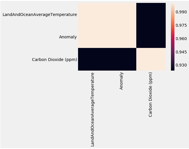

In [47]:

plt.figure(figsize=(10,8))
sns.scatterplot(x="Anomaly",y="Carbon Dioxide (ppm)", data=annual_co2_temp)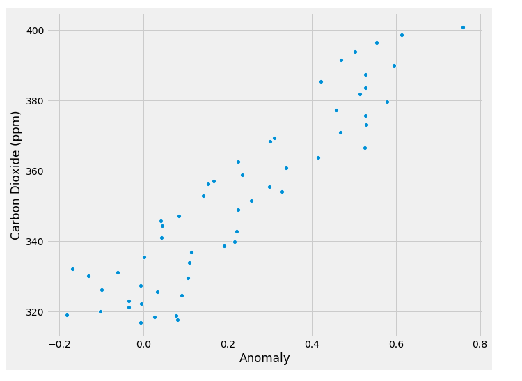

Out[47]:

<matplotlib.axes._subplots.AxesSubplot at 0x7fcace8d6c50>

With the heat map and the scatter plot, the practically linear relationship between the temperature increase and Carbon Dioxide is evident. Both are related to Climate Change. In [ ]:

undefined

The site where the data is stored has more files, for example temperature by city, to go into more detail on the situation per city. You can also keep looking for info on other countries; in the original article Greece was done, and here I tried Argentina, Brazil, Chile, Canada, Mexico and Venezuela.

Make a donation! If you liked the article you can make a donation with Bitcoin (BTC) using the digital wallet of your choice to the following address: 17MtNybhdkA9GV3UNS6BTwPcuhjXoPrSzV

Or by scanning the QR code from your wallet:

Ernesto Crespo.

Summary

Analyzing climate change data and atmospheric CO2 levels with Python and pandas.

Import the pandas, matplotlib and seaborn libraries.

Create the dataframes from the csv files.

The dataframes created.

Venezuela

Brazil

Chile

Mexico

Annual increase in the global average temperature

Venezuela.

Argentina

Brazil

Chile

Mexico

Annual CO2 levels in the Atmosphere

The relationship between CO2 and temperature is calculated.